Projective Dynamics
Mass-spring System And Implicit Method #
For node $i$ with mass $m_i$ experiencing force $\boldsymbol{f_i}$
\[\begin{align} &m_i\boldsymbol{v_i^{t+1}}=m_i\boldsymbol{v_i^{t}}+\Delta t\boldsymbol{f_i^{t+1}}\\ &\boldsymbol{x_i^{t+1}}=\boldsymbol{x_i^{t}}+\Delta t\boldsymbol{v_i^{t+1}}\\ \end{align}\]which goes to
\[\boldsymbol{x_i^{t+1}}=\boldsymbol{x_i^{t}}+\Delta t\boldsymbol{v_i^{t}}+\frac{1}{m_i}\Delta t^2\boldsymbol{f_i^{t+1}}\]Gathering all nodes we have
\[\boldsymbol{x^{t+1}}=\boldsymbol{x^{t}}+\Delta t\boldsymbol{v^{t}}+M^{-1}\Delta t^2\boldsymbol{f^{t+1}}\]where
\[\boldsymbol{x^{t+1}}=\begin{pmatrix} \boldsymbol{x_0^{t+1}}\\ \boldsymbol{x_1^{t+1}}\\ ... \end{pmatrix},\boldsymbol{v^{t+1}}=\begin{pmatrix} \boldsymbol{v_0^{t+1}}\\ \boldsymbol{v_1^{t+1}}\\ ... \end{pmatrix},\boldsymbol{f^{t+1}}=\begin{pmatrix} \boldsymbol{f_0^{t+1}}\\ \boldsymbol{f_1^{t+1}}\\ ... \end{pmatrix}\]and
\[M=\begin{pmatrix} m_0\\ &m_0\\ &&m_0\\ &&&m_1\\ &&&&m_1\\ &&&&&m_1\\ &&&&&&... \end{pmatrix}\]Considering $\boldsymbol{x^{t+1}}$ as unkown variable to be found, we have
\[\begin{align} &\boldsymbol{x}-\boldsymbol{x^{t}}-\Delta t\boldsymbol{v^{t}}-M^{-1}\Delta t^2\boldsymbol{f(x)}=\boldsymbol{0}\\ &\frac{1}{\Delta t^2}M(\boldsymbol{x}-\boldsymbol{x^{t}}-\Delta t\boldsymbol{v^{t}})-\boldsymbol{f(x)}=\boldsymbol{0} \end{align}\]Construct a function
\[F(\boldsymbol{x})=\frac{1}{2\Delta t^2}||\boldsymbol{x}-\boldsymbol{x^{t}}-\Delta t\boldsymbol{v^{t}}||^2_{M}+E(\boldsymbol{x}),\ ||a||_M^2=a^TMa\]where $\partial E/\partial \boldsymbol{x}=-\boldsymbol{f}$, we will see that
\[\begin{align} \frac{\partial F(\boldsymbol{x})}{\partial \boldsymbol{x}}&=\frac{1}{2\Delta t^2}(M+M^T)(\boldsymbol{x}-\boldsymbol{x^{t}}-\Delta t\boldsymbol{v^{t}})-\boldsymbol{f(x)}\\ &=\frac{1}{\Delta t^2}M(\boldsymbol{x}-\boldsymbol{x^{t}}-\Delta t\boldsymbol{v^{t}})-\boldsymbol{f(x)} \end{align}\]Or in some senarios we can also write it with respect to $\boldsymbol{v}$
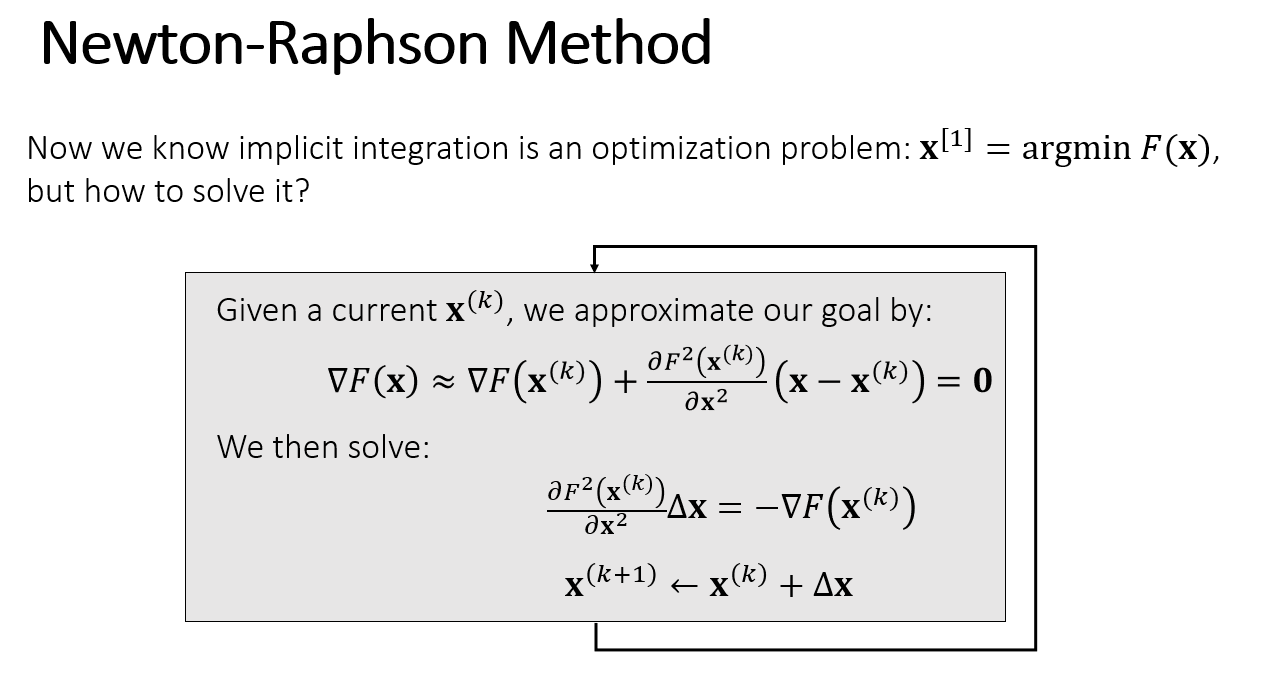
\[\begin{align} \frac{\partial F}{\partial \boldsymbol{v}}&=\frac{\partial F}{\partial \boldsymbol{x}}\frac{\partial \boldsymbol{x}}{\partial \boldsymbol{v}}=\frac{\partial F}{\partial \boldsymbol{x}}\frac{\partial (\boldsymbol{x^t}+\Delta t \boldsymbol{v})}{\partial \boldsymbol{v}}=\Delta t\frac{\partial F}{\partial \boldsymbol{x}}\\ &=\frac{1}{\Delta t}M(\boldsymbol{x}-\boldsymbol{x^{t}}-\Delta t\boldsymbol{v^{t}})-\Delta t\boldsymbol{f(x)}\\ &=M(\boldsymbol{v}-\boldsymbol{v^t})-\Delta t\boldsymbol{f(x)} \end{align}\]so we are finding $\boldsymbol{x}$ such that $\frac{\partial F(\boldsymbol{x})}{\partial \boldsymbol{x}}=0$, which is also a necessary condition for local minimum of $F$. That is, if we find a $\boldsymbol{x}$ at which $F$ is locally minimal, we find a $\boldsymbol{x}$ such that $\frac{\partial F(\boldsymbol{x})}{\partial \boldsymbol{x}}=0$. Finding local minimum can be done by Newton-Raphson’s method.
We will need to calculate the hessian of $F$.
\[\frac{\partial^2 F}{\partial \boldsymbol{x}^2}=\frac{1}{\Delta t^2}M+\partial \boldsymbol{f}/\partial \boldsymbol{x}=\frac{1}{\Delta t^2}M+H\]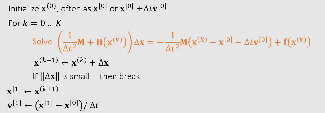
Position Based Dynamics #
High stiffness can cause problem when updating position using newton’s law (time and force). If we have another rule to directly manuplate position while conserving neccesary physical quantity (e.g. momentum), the problem can be solved. That is PBD. PBD is non-physical.
We will define the constraint as
\[C_{*}(\boldsymbol{x}) = ||\boldsymbol{x_i}-\boldsymbol{x_j}||-d\]where $d$ is the rest length between node $i$ and $j$. In general, we want all nodes satisfying constraints
\[\boldsymbol{C(x)}=\begin{pmatrix} C_0(\boldsymbol{x})\\ C_1(\boldsymbol{x})\\ ... \end{pmatrix}\]But sadly in practice, we usually cannot satisfy all constraints at once, and must iterate over all constraints. Take one constraint $C_i$ for example. If the system has experienced an external force and moved to $\boldsymbol{x^{new}}$, the constraint is still expected to be satisfied
\[\boldsymbol{C_i(x^{new})}=\boldsymbol{C_i(x+\Delta x)}\approx\boldsymbol{C_i(x)}+\frac{\partial \boldsymbol{C_i}}{\partial \boldsymbol{x}}\Delta\boldsymbol{x}=\boldsymbol{C_i(x)}+\nabla\boldsymbol{C_i}\Delta\boldsymbol{x}=\boldsymbol{0}\]Here PBD makes an assumption: the direction of $\Delta\boldsymbol{x}$ is same with gradient of $\boldsymbol{C}_i$
\[\Delta\boldsymbol{x}=\lambda(\nabla\boldsymbol{C_i})^T\]Substitute it into previous equation and we will get
\[\boldsymbol{\lambda}=-\frac{\boldsymbol{C_i}}{||\nabla \boldsymbol{C_i}||^2}\]and
\[\Delta\boldsymbol{x}=\lambda(\nabla\boldsymbol{C_i})^T=-\frac{\boldsymbol{C_i}}{||\nabla \boldsymbol{C_i}||^2}(\nabla\boldsymbol{C_i})^T\]For the correction of an individual point $\boldsymbol{x_{k}}$, we have
\[\Delta\boldsymbol{x}_k=-\frac{\boldsymbol{C_i}}{||\nabla \boldsymbol{C_i}||^2}(\nabla_{\boldsymbol{x}_k}\boldsymbol{C_i})^T=s_i(\nabla_{\boldsymbol{x}_k}\boldsymbol{C_i})^T\]where the scaling factor
\[s_i = -\boldsymbol{C_i} / ||\nabla \boldsymbol{C_i}||^2\]If the points have individual masses, we weight the corrections $\Delta\boldsymbol{x_k}$ by the inverse masses $w_k=1/m_k$
\[\Delta\boldsymbol{x}_k=\lambda w_k(\nabla_{\boldsymbol{x}_k}\boldsymbol{C_i})^T\]Finally, we have
\[s_i=\frac{\boldsymbol{C_i}}{\sum_kw_k||\nabla_{\boldsymbol{x}_k} \boldsymbol{C_i}||^2}\]and
\[\Delta\boldsymbol{x}_k=s_i w_k(\nabla_{\boldsymbol{x}_k}\boldsymbol{C_i})^T\]Following is a concrete example in one-spring case.
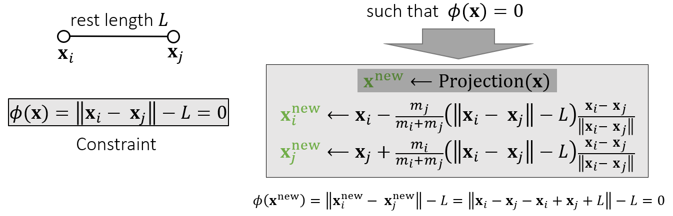
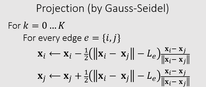
What about multiple springs? The Gauss-Seidel approach projects each spring sequentially in a certain order. We cannot ensure the satisfaction of every constraint. But the more iterations we use, the better those constraints are satisfied.
Instead of representing all the elastic potential as a penalty-like term, PBD treats all the constraints as infinitely hard constraints. For instance, in a mass-spring system simulation, PBD also treats all springs as inextensible springs.
Projective Dynamics #
For simplification, we will denote $\boldsymbol{y}:=\boldsymbol{x^{t}}+\Delta t\boldsymbol{v^{t}}$, so
\[\begin{align} F(\boldsymbol{x})&=\frac{1}{2\Delta t^2}||\boldsymbol{x}-\boldsymbol{x^{t}}-\Delta t\boldsymbol{v^{t}}||^2_{M}+E(\boldsymbol{x})\\ &=\frac{1}{2\Delta t^2}(\boldsymbol{x-y})^TM(\boldsymbol{x-y})+E(\boldsymbol{x}) \end{align}\]The optimization problem offers an interesting insight into Position Based Dynamics. If we define an energy potential EP BD as the sum of squares of the PBD constraints, we notice that the PBD constraint projection solver attempts to minimize F using a Gauss-Seidel-like method. Unfortunately, the PBD solver does not take the inertial term explicitly into account, and further the projection of each individual constraint is not guaranteed to decrease energy because the effect of the remaining constraints is ignored. Nevertheless, PBD is typically quite effective at reducing F and can be therefore understood as a heuristic variant of the implicit Euler method.
Mass-spring System #
We wll start introducing PD from simple mass-spring system containing $n$ vertices and $m$ springs.
In the first step, we wll reformulate elastic energy
\[E=\frac{k}{2}(||\boldsymbol{x_1-x_2}-r||)^2\]where $\boldsymbol{x_1,x_2}$ are spring endpoints, $r$ is the rest length, and $k$ is the spring stiffness. The key to reformulation is the following fact showing that the spring potential is a solution to a specially designed constrained minimization problem.
\[{\rm min}\ (||\boldsymbol{x}||-r)^2=\mathop{\rm min}_{||\boldsymbol{d}||=r}\ ||\boldsymbol{x}-\boldsymbol{d}||^2\]That is, from
\[{\rm min}\ F(\boldsymbol{x})={\rm min}\ \frac{1}{2\Delta t^2}(\boldsymbol{x-y})^TM(\boldsymbol{x-y})+\sum_{i=1}^m\frac{k_i}{2}(||\boldsymbol{x_{i_1}-x_{i_2}}||-r_i)^2\]we goes to
\[{\rm min}\ F(\boldsymbol{x})=\mathop{\rm min}_{||\boldsymbol{d_i}||=r_i}\ \frac{1}{2\Delta t^2}(\boldsymbol{x-y})^TM(\boldsymbol{x-y})+\sum_{i=1}^m\frac{k_i}{2}||\boldsymbol{x_{i_1}-x_{i_2}-d_i}||^2\]where $i$ indicates the i-th spring and $i_{1},i_{2}$ indicates two end points of the i-th spring.
It might sound like a bad idea to reformulate our original unconstrained minimization problem into a constrained optimization problem with an extra auxilary variable $\boldsymbol{d_i}$ which almost doubles the degrees of the freedom of the system. However, the new problem can be really easily solved by alternating optimization (also known as local-global optimization). In the local step, we fix $\boldsymbol{x}$ and find $\boldsymbol{d}$. In the global step, we fix $\boldsymbol{d}$ and find $\boldsymbol{x}$ by solving a large convex quadratic optimization problem iteratively.
\[\boldsymbol{x}=(\frac{M}{\Delta t^2}+L)^{-1}(\frac{M}{\Delta t^2}\boldsymbol{y}+J\boldsymbol{d})\]where
\[\begin{align} E(\boldsymbol{x})&=\sum_{i=1}^m\frac{k_i}{2}||\boldsymbol{x_{i_1}-x_{i_2}-d_i}||^2\\ &=\sum_{i=1}^m\frac{k_i}{2}(\boldsymbol{x_{i_1}-x_{i_2}})^T(\boldsymbol{x_{i_1}-x_{i_2}})-k_i(\boldsymbol{x_{i_1}-x_{i_2}})^T\boldsymbol{d_i}+C\\ &=\frac{1}{2}\boldsymbol{x}^TL\boldsymbol{x}-\boldsymbol{x}^TJ\boldsymbol{d}+C\\ L=&\sum_{i=1}^mk_iG_iG_i^T,\ J=\sum_{i=1}^mk_iG_iS_i^T \end{align}\]where $G_i\in R^{n\times1}$ is the incidence vector of the i-th spring, i.e. $G_i(i_1)=1$ and $G_i(i_2)=-1$ and zero otherwise. Similarly, $S_i\in R^{m\times1}$ is a indicator vector for the i-th spring, $S_i=\delta_i$. Based on this, we have
\[\begin{align} x_{i_1}-x_{i_2}=G_i^T\boldsymbol{x}\\ d_i=S_i^T\boldsymbol{d} \end{align}\]Notice here we only discuss one dimension (x/y/z). If considering 3 dimensions, we will need to do $L^3=L\otimes I_{33},G^3=G\otimes I_{33}$. $\otimes$ denotes Kronecker product. It is easy to see both $M/\Delta t^2$ and $L$ are symmetric and positive semi-definite.
ARAP Material #
We start from how to calculate deformation gradient $F$ for a tetrahedron with 4 vertices $\boldsymbol{x_1,x_2,x_3,x_4}$ in deformed state and $\boldsymbol{X_1,X_2,X_3,X_4}$ in reference state . We know that
\[\begin{align} \boldsymbol{x_1-x_4}&=F(\boldsymbol{X_1-X_4})\\ \boldsymbol{x_2-x_4}&=F(\boldsymbol{X_2-X_4})\\ \boldsymbol{x_3-x_4}&=F(\boldsymbol{X_3-X_4})\\ \end{align}\]So $F=D_sD_m^{-1}$ where $D_s=[\boldsymbol{x_1-x_4};\boldsymbol{x_2-x_4};\boldsymbol{x_3-x_4}]$ and $D_m=[\boldsymbol{X_1-X_4};\boldsymbol{X_2-X_4};\boldsymbol{X_3-X_4}]$.
For an object containing $m$ tetrahedrons and $n$ vertices, we denote $F_i^T=D_{mi}^{-T}D_{si}^T$ for i-th tetrahedron where $D_{si}^T\in R^{3\times3}$ can be represented as a linear combination of the position vector $\boldsymbol{x}$ (note here $\boldsymbol{x} \in R^{n\times 3}$ is different from above in $R^{3n\times 1}$) as $D_{si}^T=A_i\boldsymbol{x}$ where
\[A_i=\begin{bmatrix} ...&1&...&0&...&0&...&-1&...\\ ...&0&...&1&...&0&...&-1&...\\ ...&0&...&0&...&1&...&-1&...\\ \end{bmatrix}\]where the non-zero columns are corresponding to the indices of the first second third and fourth vertex of the i-th element. If we denote $G_i^T=D_{mi}^{-T}A_i$ then $F_i^T=G_i^T\boldsymbol{x}$.
Consider we now define potential density as
\[\psi(F(\boldsymbol{x}))=\mathop{\rm min}_{p\in SO(3)}||F-p||_F^2=||F-R||_F^2\]where $F=RS$ is the polar decomposition of $F$. So the potential is equivalent with ARAP. Then
\[E(\boldsymbol{x})=\frac{1}{2}\sum_iV_ik_i\mathop{\rm min}_{p\in SO(3)}||F_i-p_i||_F^2=\frac{1}{2}\sum_iV_ik_i\mathop{\rm min}_{p\in SO(3)}||F_i^T-p_i^T||_F^2\]$p_i$ can also be represented with selector matrix $p_i=S_i^T\boldsymbol{p}$ where $\boldsymbol{p}\in R^{3m\times3}$ is the stacked version of $p_i$. And $S_i=\delta_i\otimes I_{33}\in R^{3m\times 3}$.
So the energy can be rewritten in
\[\begin{align} E(\boldsymbol{x})&=\frac{1}{2}\sum_iV_ik_i\mathop{\rm min}_{p\in SO(3)}||G_i^T\boldsymbol{x}-S_i^T\boldsymbol{p}||_F^2\\ &=\mathop{\rm min}_{p\in SO(3)}\frac{1}{2}{\rm tr}(\boldsymbol{x^T}L\boldsymbol{x})-{\rm tr}(\boldsymbol{x^T}J\boldsymbol{p})+C\\ L=&\sum_{i=1}^mV_ik_iG_iG_i^T,\ J=\sum_{i=1}^mV_ik_iG_iS_i^T \end{align}\]Gradient Descent #